Facets (ggplot2)
Problem
You want to do split up your data by one or more variables and plot the subsets of data together.
Solution
Sample data
We will use the tips dataset from the reshape2 package.
library(reshape2)
# Look at first few rows
head(tips)
#>   total_bill  tip    sex smoker day   time size
#> 1      16.99 1.01 Female     No Sun Dinner    2
#> 2      10.34 1.66   Male     No Sun Dinner    3
#> 3      21.01 3.50   Male     No Sun Dinner    3
#> 4      23.68 3.31   Male     No Sun Dinner    2
#> 5      24.59 3.61 Female     No Sun Dinner    4
#> 6      25.29 4.71   Male     No Sun Dinner    4
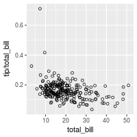
This is a scatterplot of the tip percentage by total bill size.
library(ggplot2)
sp <- ggplot(tips, aes(x=total_bill, y=tip/total_bill)) + geom_point(shape=1)
sp
facet_grid
The data can be split up by one or two variables that vary on the horizontal and/or vertical direction.
This is done by giving a formula to facet_grid(), of the form vertical ~ horizontal.
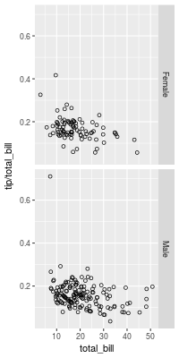
# Divide by levels of "sex", in the vertical direction
sp + facet_grid(sex ~ .)
# Divide by levels of "sex", in the horizontal direction
sp + facet_grid(. ~ sex)

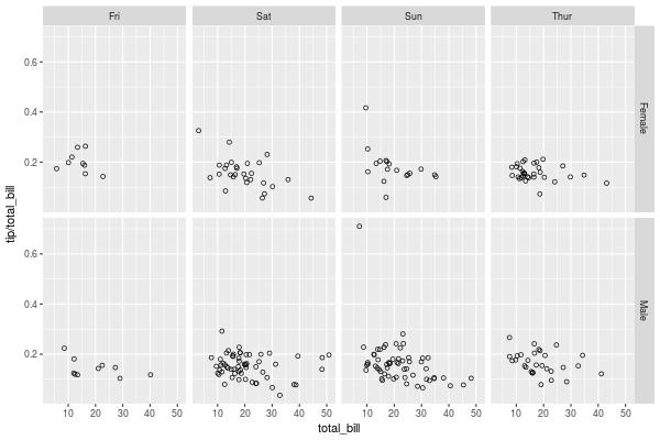
# Divide with "sex" vertical, "day" horizontal
sp + facet_grid(sex ~ day)
facet_wrap
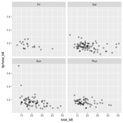
Instead of faceting with a variable in the horizontal or vertical direction, facets can be placed next to each other, wrapping with a certain number of columns or rows. The label for each plot will be at the top of the plot.
# Divide by day, going horizontally and wrapping with 2 columns
sp + facet_wrap( ~ day, ncol=2)
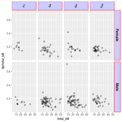
Modifying facet label appearance
sp + facet_grid(sex ~ day) +
    theme(strip.text.x = element_text(size=8, angle=75),
          strip.text.y = element_text(size=12, face="bold"),
          strip.background = element_rect(colour="red", fill="#CCCCFF"))
Modifying facet label text
There are a few different ways of modifying facet labels. The simplest way is to provide a named vector that maps original names to new names. To map the levels of sex from Female==>Women, and Male==>Men:
labels <- c(Female = "Women", Male = "Men")
sp + facet_grid(. ~ sex, labeller=labeller(sex = labels))
Another way is to modify the data frame so that the data contains the desired labels:
tips2 <- tips
levels(tips2$sex)[levels(tips2$sex)=="Female"] <- "Women"
levels(tips2$sex)[levels(tips2$sex)=="Male"]   <- "Men"
head(tips2, 3)
#>   total_bill  tip   sex smoker day   time size
#> 1      16.99 1.01 Women     No Sun Dinner    2
#> 2      10.34 1.66   Men     No Sun Dinner    3
#> 3      21.01 3.50   Men     No Sun Dinner    3

# Both of these will give the same output:
sp2 <- ggplot(tips2, aes(x=total_bill, y=tip/total_bill)) + geom_point(shape=1)
sp2 + facet_grid(. ~ sex)
Both of these will give the same result:

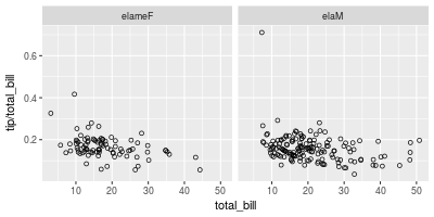
labeller() can use any function that takes a character vector as input and returns a character vector as output. For example, the capitalize function from the Hmisc package will capitalize the first letters of strings. We can also define our own custom functions, like this one, which reverses strings:
# Reverse each strings in a character vector
reverse <- function(strings) {
    strings <- strsplit(strings, "")
    vapply(strings, function(x) {
        paste(rev(x), collapse = "")
    }, FUN.VALUE = character(1))
}

sp + facet_grid(. ~ sex, labeller=labeller(sex = reverse))
Free scales
Normally, the axis scales on each graph are fixed, which means that they have the same size and range. They can be made independent, by setting scales to free, free_x, or free_y.
# A histogram of bill sizes
hp <- ggplot(tips, aes(x=total_bill)) + geom_histogram(binwidth=2,colour="white")
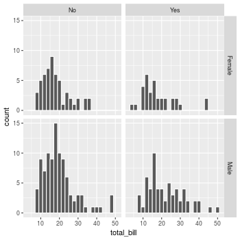
# Histogram of total_bill, divided by sex and smoker
hp + facet_grid(sex ~ smoker)
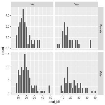
# Same as above, with scales="free_y"
hp + facet_grid(sex ~ smoker, scales="free_y")
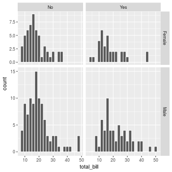
# With panels that have the same scaling, but different range (and therefore different physical sizes)
hp + facet_grid(sex ~ smoker, scales="free", space="free")