Calculating a moving average
Problem
You want to calculate a moving average.
Solution
Suppose your data is a noisy sine wave with some missing values:
set.seed(993)
x <- 1:300
y <- sin(x/20) + rnorm(300,sd=.1)
y[251:255] <- NA
The filter() function can be used to calculate a moving average.
# Plot the unsmoothed data (gray)
plot(x, y, type="l", col=grey(.5))
# Draw gridlines
grid()

# Smoothed with lag:
# average of current sample and 19 previous samples (red)
f20 <- rep(1/20, 20)
f20
#>  [1] 0.05 0.05 0.05 0.05 0.05 0.05 0.05 0.05 0.05 0.05 0.05 0.05 0.05 0.05 0.05 0.05 0.05
#> [18] 0.05 0.05 0.05
y_lag <- filter(y, f20, sides=1)
lines(x, y_lag, col="red")

# Smoothed symmetrically:
# average of current sample, 10 future samples, and 10 past samples (blue)
f21 <- rep(1/21,21)
f21
#>  [1] 0.04761905 0.04761905 0.04761905 0.04761905 0.04761905 0.04761905 0.04761905
#>  [8] 0.04761905 0.04761905 0.04761905 0.04761905 0.04761905 0.04761905 0.04761905
#> [15] 0.04761905 0.04761905 0.04761905 0.04761905 0.04761905 0.04761905 0.04761905
y_sym <- filter(y, f21, sides=2)
lines(x, y_sym, col="blue")
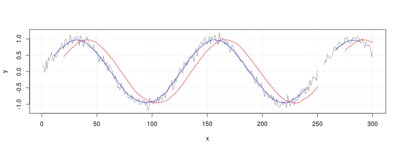
filter() will leave holes wherever it encounters missing values, as shown in the graph above.
A different way to handle missing data is to simply ignore it, and not include it in the average. The function defined here will do that.
# x: the vector
# n: the number of samples
# centered: if FALSE, then average current sample and previous (n-1) samples
# if TRUE, then average symmetrically in past and future. (If n is even, use one more sample from future.)
movingAverage <- function(x, n=1, centered=FALSE) {
if (centered) {
before <- floor ((n-1)/2)
after <- ceiling((n-1)/2)
} else {
before <- n-1
after <- 0
}
# Track the sum and count of number of non-NA items
s <- rep(0, length(x))
count <- rep(0, length(x))
# Add the centered data
new <- x
# Add to count list wherever there isn't a
count <- count + !is.na(new)
# Now replace NA_s with 0_s and add to total
new[is.na(new)] <- 0
s <- s + new
# Add the data from before
i <- 1
while (i <= before) {
# This is the vector with offset values to add
new <- c(rep(NA, i), x[1:(length(x)-i)])
count <- count + !is.na(new)
new[is.na(new)] <- 0
s <- s + new
i <- i+1
}
# Add the data from after
i <- 1
while (i <= after) {
# This is the vector with offset values to add
new <- c(x[(i+1):length(x)], rep(NA, i))
count <- count + !is.na(new)
new[is.na(new)] <- 0
s <- s + new
i <- i+1
}
# return sum divided by count
s/count
}
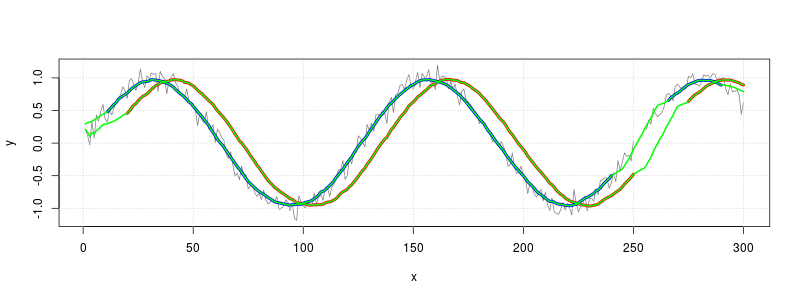
# Make same plots from before, with thicker lines
plot(x, y, type="l", col=grey(.5))
grid()
y_lag <- filter(y, rep(1/20, 20), sides=1)
lines(x, y_lag, col="red", lwd=4) # Lagged average in red
y_sym <- filter(y, rep(1/21,21), sides=2)
lines(x, y_sym, col="blue", lwd=4) # Symmetrical average in blue
# Calculate lagged moving average with new method and overplot with green
y_lag_na.rm <- movingAverage(y, 20)
lines(x, y_lag_na.rm, col="green", lwd=2)
# Calculate symmetrical moving average with new method and overplot with green
y_sym_na.rm <- movingAverage(y, 21, TRUE)
lines(x, y_sym_na.rm, col="green", lwd=2)